4 Interactive graph

Code

#install.packages("alr4")
library(ggplot2)
library(dplyr)


Attaching package: 'dplyr'

The following objects are masked from 'package:stats':

    filter, lag

The following objects are masked from 'package:base':

    intersect, setdiff, setequal, union

Code

#install.packages("broom")
library(broom)  
library(tidyverse)

── Attaching core tidyverse packages ──────────────────────── tidyverse 2.0.0 ──
✔ forcats   1.0.0     ✔ stringr   1.5.1
✔ lubridate 1.9.4     ✔ tibble    3.2.1
✔ purrr     1.0.2     ✔ tidyr     1.3.1
✔ readr     2.1.5

── Conflicts ────────────────────────────────────────── tidyverse_conflicts() ──
✖ dplyr::filter() masks stats::filter()
✖ dplyr::lag()    masks stats::lag()
ℹ Use the conflicted package (<http://conflicted.r-lib.org/>) to force all conflicts to become errors

Code

library(alr4)

Loading required package: car
Loading required package: carData

Attaching package: 'car'

The following object is masked from 'package:purrr':

    some

The following object is masked from 'package:dplyr':

    recode

Loading required package: effects
lattice theme set by effectsTheme()
See ?effectsTheme for details.

Code

data(Highway)
str(Highway)

'data.frame':   39 obs. of  12 variables:
 $ adt  : int  69 73 49 61 28 30 46 25 43 23 ...
 $ trks : int  8 8 10 13 12 6 8 9 12 7 ...
 $ lane : int  8 4 4 6 4 4 4 4 4 4 ...
 $ acpt : num  4.6 4.4 4.7 3.8 2.2 24.8 11 18.5 7.5 8.2 ...
 $ sigs : num  0 0 0 0 0 1.84 0.7 0.38 1.39 1.21 ...
 $ itg  : num  1.2 1.43 1.54 0.94 0.65 0.34 0.47 0.38 0.95 0.12 ...
 $ slim : int  55 60 60 65 70 55 55 55 50 50 ...
 $ len  : num  4.99 16.11 9.75 10.65 20.01 ...
 $ lwid : int  12 12 12 12 12 12 12 12 12 12 ...
 $ shld : int  10 10 10 10 10 10 8 10 4 5 ...
 $ htype: Factor w/ 4 levels "mc","fai","pa",..: 2 2 2 2 2 3 3 3 3 3 ...
 $ rate : num  4.58 2.86 3.02 2.29 1.61 6.87 3.85 6.12 3.29 5.88 ...

Code

model_1 <- lm(rate ~ trks + acpt, data = Highway)
summary(model_1)


Call:
lm(formula = rate ~ trks + acpt, data = Highway)

Residuals:
    Min      1Q  Median      3Q     Max 
-2.0610 -0.9655  0.1222  0.6568  3.1717 

Coefficients:
            Estimate Std. Error t value Pr(>|t|)    
(Intercept)  4.42932    1.00856   4.392 9.47e-05 ***
trks        -0.23418    0.09134  -2.564   0.0147 *  
acpt         0.13896    0.02308   6.021 6.52e-07 ***
---
Signif. codes:  0 '***' 0.001 '**' 0.01 '*' 0.05 '.' 0.1 ' ' 1

Residual standard error: 1.237 on 36 degrees of freedom
Multiple R-squared:  0.6326,    Adjusted R-squared:  0.6122 
F-statistic: 30.99 on 2 and 36 DF,  p-value: 1.487e-08

Code

model_2 <- lm(rate ~ slim, data = Highway)
summary(model_2)


Call:
lm(formula = rate ~ slim, data = Highway)

Residuals:
    Min      1Q  Median      3Q     Max 
-2.3295 -0.9653 -0.2072  0.7297  4.2767 

Coefficients:
            Estimate Std. Error t value Pr(>|t|)    
(Intercept) 16.65103    2.26068   7.366 9.29e-09 ***
slim        -0.23123    0.04088  -5.657 1.83e-06 ***
---
Signif. codes:  0 '***' 0.001 '**' 0.01 '*' 0.05 '.' 0.1 ' ' 1

Residual standard error: 1.474 on 37 degrees of freedom
Multiple R-squared:  0.4637,    Adjusted R-squared:  0.4492 
F-statistic:    32 on 1 and 37 DF,  p-value: 1.833e-06

Code

full_model <- lm(rate ~ trks + acpt + slim, data = Highway)
summary(full_model)


Call:
lm(formula = rate ~ trks + acpt + slim, data = Highway)

Residuals:
    Min      1Q  Median      3Q     Max 
-2.3652 -0.9490  0.1412  0.7481  2.4973 

Coefficients:
            Estimate Std. Error t value Pr(>|t|)    
(Intercept) 10.20690    2.79157   3.656 0.000833 ***
trks        -0.21994    0.08705  -2.527 0.016195 *  
acpt         0.09815    0.02871   3.419 0.001613 ** 
slim        -0.09844    0.04467  -2.204 0.034222 *  
---
Signif. codes:  0 '***' 0.001 '**' 0.01 '*' 0.05 '.' 0.1 ' ' 1

Residual standard error: 1.175 on 35 degrees of freedom
Multiple R-squared:  0.6774,    Adjusted R-squared:  0.6497 
F-statistic:  24.5 on 3 and 35 DF,  p-value: 1.014e-08

Code

r2_model_1 <- summary(model_1)$r.squared
r2_model_2 <- summary(model_2)$r.squared
r2_full_model <- summary(full_model)$r.squared

print(r2_model_1)

[1] 0.6326149

Code

print(r2_model_2)

[1] 0.4637387

Code

print(r2_full_model)

[1] 0.6773765

We can find that \(R^2\) from the model 1 is 0.6326149, \(R^2\) from the model 2 is 0.4637387 and \(R^2\) from the full model is 0.6773765. Certainly \(R^2\) from the model 1 much more closer to full model. So we can find that trks and acpt are more important in model. Slim does not significantly improve the model.

How much additional variation is explained by the addition of slim to model 1?

Code

0.6773765-0.6326149

[1] 0.0447616

Almost 0.0447616 additional variation is explained by the addition of slim to model 1.

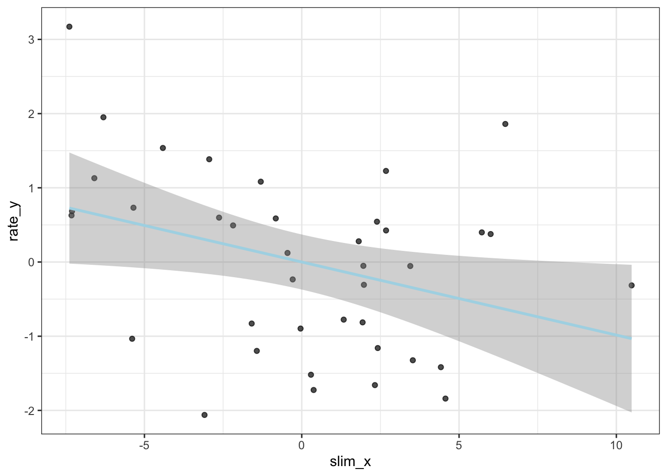
Create an added variable plot for slim and add the best fitting line. (Hint: unlike the example in class, there are two other regressors in the problem besides slim.)

Code

rate_y <- residuals(lm(rate ~ trks + acpt, data = Highway))
slim_x <- residuals(lm(slim ~ trks + acpt, data = Highway))

avp_data <- data.frame(rate_y, slim_x)

ggplot(avp_data, aes(x = slim_x, y = rate_y)) +
  geom_point(alpha = 0.7) +
  geom_smooth(method = "lm", color = "lightblue") +
  theme_bw()

`geom_smooth()` using formula = 'y ~ x'